The Simulator Is the Reward: Building LLM Agents for Physical Engineering Domains

There is a class of software that millions of engineers use every day. It generates rich, deterministic, physically grounded feedback, and the LLM agent community has almost ignored it: domain-specific simulation tools. SPICE for circuit design. ANSYS for structural mechanics. Cadence for chip layout. Zemax for optics.

These tools are not just interfaces. They are reward machines, and that has real implications for how we build agents on top of them.

The engineer’s loop

Before writing a single line of agent code, it is worth understanding what engineers actually do. The workflow is surprisingly uniform across domains.

Imagine a mixed-signal IC designer working on an amplifier. They start with a specification: gain of 40 dB, bandwidth of 1 GHz, power budget of 10 mW, input noise below 5 nV/√Hz. They then do what every experienced engineer does and reach for a known topology. A cascode? A folded-cascode OTA? The choice comes from years of pattern matching against past designs, textbooks, application notes, and the informal knowledge that circulates in design reviews.

Once they have a starting topology, they build the circuit in their simulator, assign initial component values, run an AC analysis, and look at the Bode plot. The gain is 36 dB instead of 40. The bandwidth is fine. The noise is slightly over budget. So they adjust: maybe increase the tail current, swap a device for a higher-gm variant, tweak the load resistance. Then they simulate again.

This is the loop: propose → simulate → interpret → adjust → repeat.

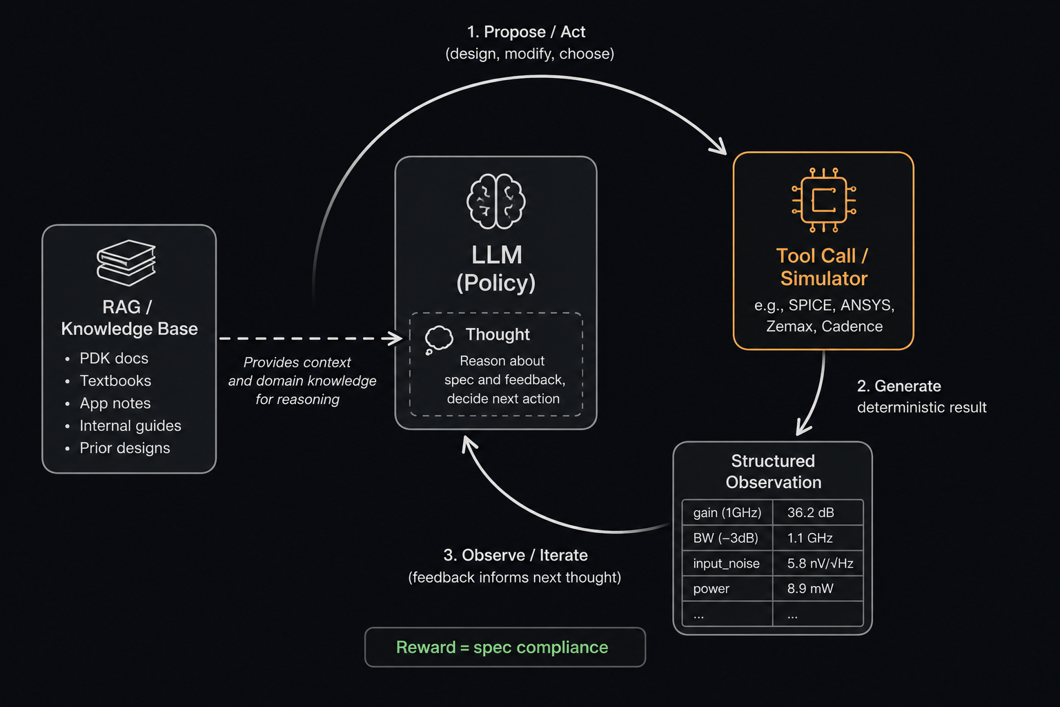
Two things are worth noting about this loop. First, the proposal step is heavily loaded with tacit knowledge, the heuristics that experts cannot always fully articulate but that consistently produce reasonable starting points. Second, the simulation step is completely deterministic: given a circuit, the physics gives you back a unique, unambiguous result. There is no labeling, no annotation, no human judgment required to evaluate the output.

Mapping the loop to a ReAct agent

The ReAct framework (Reason + Act) maps almost trivially onto this workflow.

Thought: The spec asks for 40 dB gain at 1 GHz. A cascode topology with
         a 5 mA tail current and PMOS loads is a reasonable starting point
         for this process node.

Action: spice_simulate(netlist=<cascode_v1.sp>, analyses=["ac", "noise"])

Observation: gain=36.2dB at 1GHz, BW=1.1GHz, input_noise=5.8nV/√Hz,
             power=8.9mW

Thought: Gain is 3.8 dB short. The noise is over budget. Increasing tail
         current will help gain but worsen power and likely hurt noise.
         Better to increase gm by widening M1/M2 by 20% first.

Action: modify_netlist(changes={"W_M1": "120u", "W_M2": "120u"})
        spice_simulate(...)

Observation: gain=38.9dB, BW=980MHz, input_noise=4.9nV/√Hz, power=9.1mW
...

The simulator tool is called on every iteration. The LLM reads the structured output (numbers, not prose) and reasons about what to change and why. Critically, this loop can run without any human in the iteration. The engineer sets the spec and reviews the final result; the agent handles the middle.

This is already useful, but two failure modes appear quickly in practice.

Failure mode 1: the initial proposal is bad. If the LLM proposes a topology that is fundamentally mismatched to the spec (wrong architecture, wrong process corner assumptions), the optimization loop will struggle or fail to recover. A bad starting point in a non-convex design space is hard to escape.

Failure mode 2: the action after simulation is unreasonable. The LLM reads a noise figure and decides to reduce load resistance, which actually makes things worse. Or it makes a change that violates a design rule it was never told about. The reasoning step is the weakest link.

Context engineering: RAG for initial proposals

When the LLM is about to propose an initial topology, it should be able to retrieve relevant context: application notes for this process node, datasheet recommendations for similar specs, internal design guides. When it reads a simulation result and needs to decide what to change, it should be able to pull in knowledge about how specific parameters affect specific outputs in this domain.

Concretely, for the circuit design case, your RAG corpus might include:

• Process design kit (PDK) documentation
• Analog design textbooks (Razavi, Allen & Holberg)
• Internal design review notes and post-mortems
• Prior successful designs with their final parameter sets

The key insight is that RAG patches failure mode 1 more reliably than failure mode 2. It gives the LLM better priors for initial proposals, because the knowledge needed for that is largely static and document-resident. The dynamic, feedback-driven adjustment reasoning is harder to capture in a document. That requires something else.

RLVR: when the simulator is the reward model

The second failure mode, unreasonable actions given simulation feedback, is fundamentally a policy alignment problem. The LLM’s default policy, trained on internet text, does not know that increasing tail current in a cascode has a specific, predictable effect on noise and gain in a specific process. This is the kind of knowledge that only emerges from doing, not reading.

This is precisely the setting that Reinforcement Learning from Verifiable Rewards (RLVR) was designed for. The term was popularized by work on mathematical reasoning (DeepSeek-R1 and others), where a math problem has a ground-truth answer that can be verified without a human. The insight transfers directly: a circuit specification has a ground-truth simulation result, and meeting the spec is a verifiable signal, whether binary or continuous.

In the RLVR framing:

• The policy is the LLM generating design actions
• The environment is the simulator
• The reward is how well the final design meets the spec (a weighted combination of gain error, noise margin, and power headroom)
• No human labeling is required anywhere in the training loop

This is a cleaner RL setup than most. The reward is deterministic, fast to compute, and physically meaningful. Noise-free rewards are notoriously good for policy gradient methods.

GRPO (Group Relative Policy Optimization, from DeepSeekMath) is the natural training algorithm here. For each design spec, sample G candidate trajectories from the current policy, evaluate each against the simulator, compute relative advantages within the group, and update the policy. Recent work on optical lens design (OPTIAGENT, arXiv 2602.23761) validates this exact setup: training a Qwen3-4B model with GRPO on simulation feedback outperforms GPT-4-class models using in-context learning, and does so with a 60x smaller model.

The catch is cost. GRPO requires thousands of rollouts, each of which involves calling the simulator. For a fast SPICE simulation (sub-second) this is tractable. For a finite element structural simulation that takes 20 minutes per run, it is not. And even in the fast case, you need GPU infrastructure to update model weights, a significant operational investment for a team made up of domain engineers rather than ML researchers.

GEPA: cheaper RL, better interpretability

GEPA (arXiv 2507.19457, ICLR 2026 Oral) offers a different path to the same destination. Instead of updating model weights via policy gradients, GEPA optimizes the prompt using natural language reflection.

The mechanism works like this. GEPA samples trajectories from the current policy, just as GRPO does. But instead of computing a gradient from scalar rewards, it asks a meta-LLM to reflect in natural language on why some trajectories succeeded and others failed. These reflections are distilled into explicit rules (“when bandwidth is within spec but gain is short, prefer increasing gm over increasing supply current”), which are then proposed as prompt updates. The Pareto frontier of past attempts is maintained so that complementary lessons, some about initial topology and some about adjustment strategy, can be combined.

The result is a prompt that encodes accumulated engineering heuristics in readable text. Empirically, GEPA outperforms GRPO by 6% on average and up to 20% on harder tasks, while using up to 35x fewer rollouts. Just as important, it requires no GPU training infrastructure, only API calls.

For physical engineering domains, GEPA has an advantage beyond cost: interpretability.

In most ML applications, interpretability is a nice-to-have. In engineering, it is often a requirement. An evolved prompt that says “for low-noise amplifier design in 28nm CMOS, start with a common-gate input stage when input impedance matching is required” is something a senior engineer can read, validate, and approve. A fine-tuned model weight is not. In regulated industries, in safety-critical applications, and in organizations where the engineering team owns the system while the ML team is a service function, readable and auditable optimization rules are not just convenient. They may be the only path to deployment.

The practical decision comes down to a few questions:

• Fast simulators, GPU infrastructure, and enough rollout budget? Use GRPO (or DrGRPO for stability).
• Slow simulations, no ML training infrastructure, or interpretability matters? Use GEPA.
• In both cases, RAG is not an alternative to either. It is a complementary component that handles the static knowledge retrieval that neither RL method specializes in.

What this looks like end to end

Putting it together for our circuit design agent:

1. Engineer provides a spec (gain, bandwidth, noise, power)
2. RAG retrieves relevant topology guides and prior designs from the knowledge base
3. LLM proposes an initial circuit, enriched by retrieved context
4. Simulator returns AC, noise, and power results
5. LLM reasons about the delta between results and spec, then decides the next modification
6. Loop continues until convergence or the iteration budget is exhausted
7. GEPA (or GRPO) optimizes steps 3 and 5, the proposal and the action, using simulation outcomes as the reward signal, with no human-labeled training data

The simulator, which used to be just a tool the engineer pointed at a design they already knew, becomes the training signal for a policy that learns how to design.

Where this breaks down

This framing has real limits worth naming.

Reward shaping is non-trivial. A spec has multiple objectives with complex trade-offs. A scalar reward that combines gain error, noise margin, power headroom, and area into a single number requires design choices that encode engineering judgment. Get the weights wrong and the agent optimizes for the wrong thing. This is the merit function problem, and it is genuinely hard.

Initial structure still matters. Both GRPO and GEPA optimize the policy, but they cannot fully compensate for a catastrophically bad starting point. In highly non-convex design spaces, the initial proposal step remains the fragile link, and RAG has limits of its own: it can only retrieve what already exists in the corpus.

Simulator fidelity matters more than it seems. A fast-but-approximate simulator is good for training but may produce an agent that learns to exploit the approximations rather than solve the real problem. Transfer from training simulator to production simulator is a real concern.

None of these are blockers. They are engineering problems with engineering solutions. But they are worth surfacing before writing the first line of code.

Closing thought

There are domains where the ground truth is hard to define, human judgment is irreplaceable, and reward signals are expensive to construct. Large parts of NLP used to be this way, before RLHF.

Physical simulation domains are not like this. The ground truth is physics. The reward signal is already built. The environment has been running deterministically for decades, waiting for someone to put an agent in the loop.

The tooling is now there. The framework is clear. The main thing left is to build it.